without haste but without rest
03. Visualization with Seabron 본문
0. 개요
-박스 플롯 - 분산 확인
-바이올린 플롯 - 분산 확인 + 분포 확인
-스캐터 플롯 - 변수들 간의 상관관계
-페어 플롯 - 변수들 간의 상관관계
-히트맵 - 변수들 간의 상관관계
-조인트 플롯 - 스캐터 + 러그
-스왐 플롯 - 분류 문제
-스트립 플롯 - 분류 문제
1. 데이터 로드
""" Exploring """
import pandas as pd

# load iris
iris = pd.read_csv("iris.csv")
iris.head()

print(iris.columns)
print(iris)
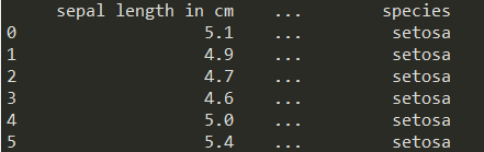
컬럼 네임들이 짤려서 나온다.
# 컬럼 이름 변경하기
iris.rename(columns = {iris.columns[0] : 'Sepal.Length',
                       iris.columns[1] : 'Sepal.Width',
                       iris.columns[2] : 'Petal.Length',
                       iris.columns[3] : 'Petal.Width',
                       iris.columns[4] : 'Species'},
                       inplace = True)
print(iris)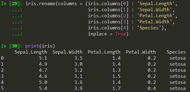
# 데이터 정보 요약
iris.describe().transpose()


# 타겟 데이터의 종류별 개수
iris['Species'].value_counts()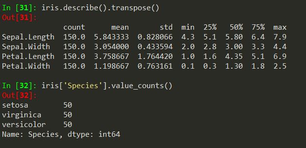
2. seaborn: dist plot
""" Visualizin: distribution """
import seaborn as sns
# style = 바탕화면 이미지, palette = 컬러 스타일 , color_codes = 팔레트 사용 여부
sns.set(style = "white", palette = "muted", color_codes = True)
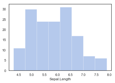
# Plot a simple histogram with binsize determined automatically
sns.distplot(iris['Sepal.Length'], kde = False, color = "b")
"""
kde 옵션은 히스토그램 라인
"""
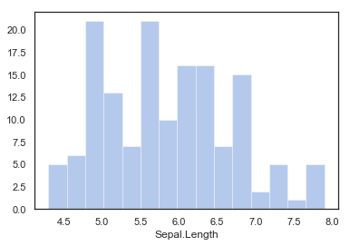
# bins / r의 breaks 옵션과 같다.
sns.distplot(iris['Sepal.Length'], bins = 15, kde = False, color = "b")
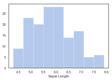
# bins의 크기를 구하는 방법 1 sturges가 제안한 방법
sns.distplot(iris['Sepal.Length'], bins = 'sturges', kde = False, color = "b")
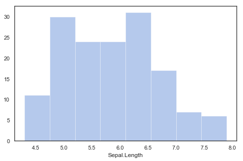
# 방법2 프리드만 다이아코니스가 제안한 방법이다
# bins 옵션의 디폴트 값이기도 하다

sns.distplot(iris['Sepal.Length'], bins = 'fd', kde = False, color = "b")
3. maplotlib: dist plot
import matplotlib.pyplot as plt

plt.figure(figsize = (8, 5))
sns.distplot(iris['Sepal.Length'], kde = False, color = "b")
plt.show()
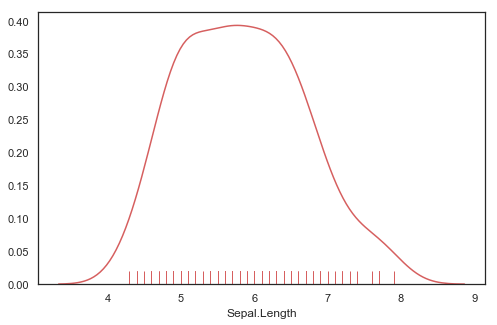
# 개별 변수에 대한 시각화 방법

# rug는 차트 밑에 |||| 형태들로 자료가 고르게 분포하는지 확인 가능

# Plot a kernel density estimate and rug plot
plt.figure(figsize = (8, 5))
sns.distplot(iris['Sepal.Length'], hist = False, rug = True, color="r")
plt.show()
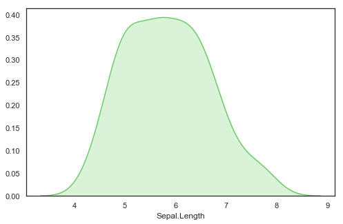
# kde_kws 옵션
# Plot a filled kernel density estimate
plt.figure(figsize = (8, 5))
sns.distplot(iris['Sepal.Length'], hist = False, color = "g", kde_kws = {"shade": True})
plt.show()
# Plot a histogram and kernel density estimate
plt.figure(figsize = (8, 5))
sns.distplot(iris['Sepal.Length'], color = "m")
plt.show()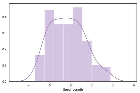
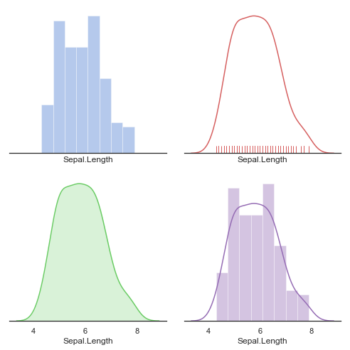
4. plot array
R의 par(mfrow=c(a, b) ) 함수와 동일
plt.subplots 메소드
""" plot array 1 """
f, axes = plt.subplots(2, 2, figsize = (7, 7), sharex = True)
sns.despine(left = True)

sns.distplot(iris['Sepal.Length'], kde = False, color = "b", ax = axes[0, 0])

sns.distplot(iris['Sepal.Length'], hist = False, rug = True, color="r", ax = axes[0, 1])

sns.distplot(iris['Sepal.Length'], hist = False, color = "g", kde_kws = {"shade": True}, ax = axes[1, 0])

sns.distplot(iris['Sepal.Length'], color = "m", ax = axes[1, 1])

plt.setp(axes, yticks = [])
plt.tight_layout()
plt.show()
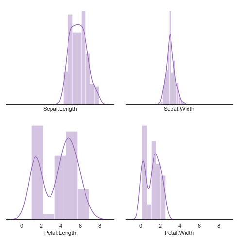
""" plot array 2 """
f, axes = plt.subplots(2, 2, figsize = (7, 7), sharex = True)
sns.despine(left = True)

# sepal.length가 petal.length보다 평균이 크고
# petal.length 가 분산이 더 큰 것을 그림으로 쉽게 파악 가능
# petal.length에는 two bimodal 이 존재한다.
# 이것만으로도 분류가 쉽게 가능하지 않을까?
sns.distplot(iris['Sepal.Length'], color = "m", ax = axes[0, 0])
sns.distplot(iris['Sepal.Width'], color = "m", ax = axes[0, 1])
sns.distplot(iris['Petal.Length'], color = "m", ax = axes[1, 0])
sns.distplot(iris['Petal.Width'], color = "m", ax = axes[1, 1])

plt.setp(axes, yticks = [])
plt.tight_layout()
plt.show()
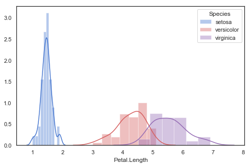
5. 멀티플 히스토그램
# 멀티플 히스토그램
""" multiple histograms on the same axis """
iris[iris['Species'] == 'setosa']

plt.figure(figsize = (8, 5))

sns.distplot(iris[iris['Species'] == 'setosa']['Petal.Length'], color = "b", label = 'setosa')
sns.distplot(iris[iris['Species'] == 'versicolor']['Petal.Length'], color = "r", label = 'versicolor')
sns.distplot(iris[iris['Species'] == 'virginica']['Petal.Length'], color = "m", label = 'virginica')

plt.legend(title = "Species")

plt.show()
# 멀티플 히스토그램을 통계학적 관점에서 살펴보는 방법
# 박스 플롯


""" box plot """
plt.figure(figsize = (8, 5))

sns.boxplot(x = 'Petal.Length', y = 'Species', data = iris)

plt.show()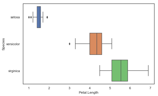
6. 두 개 이상의 변수들의 관계 살펴보기
# 피쳐들이 서로 어떤 관계를 가지고 있는가?
# 둘 이상의 변수에서의 관계 살펴보기
""" scatter plot 1 """
plt.figure(figsize = (8, 8))

sns.scatterplot(x = 'Petal.Length', y = 'Petal.Width', data = iris)

plt.show()

컬러 구분이 안 되어 있어서 구분하기가 어렵다.
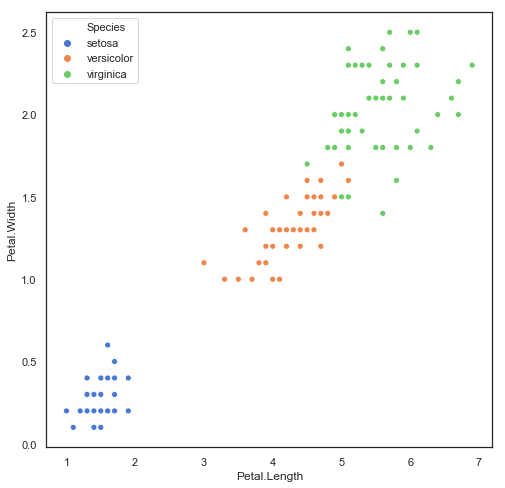
# 컬러링을 이용해서 색 추가
# *hue 옵션은 그룹별로 컬러링하는 옵션이다.

""" scatter plot 2: coloring """
plt.figure(figsize = (8, 8))

sns.scatterplot(x = 'Petal.Length', y = 'Petal.Width', hue = 'Species', data = iris)

plt.show()
회귀 선 추가하기
"""
세토사의 경우 데이터의 분포만으로도 분류할 수 있을 것 같다.
하지만 버지칼라와 버지니카는 분포가 섞여있다.
그런데 두 품종의 petal.length, petal.width 간의 관계의 상관계수가
차이를 보인다.

따라서 절편을 통해서 두 품종을 구분할 수 있지 않을까 생각해볼 수 있다.

"""

""" scatter plot 2: regression line """
g = sns.lmplot(x = 'Petal.Length', y = 'Petal.Width', hue = 'Species', height = 6, aspect = 8 / 6,  data = iris)

g.set_axis_labels("Pepal length (mm)", "Pepal width (mm)")

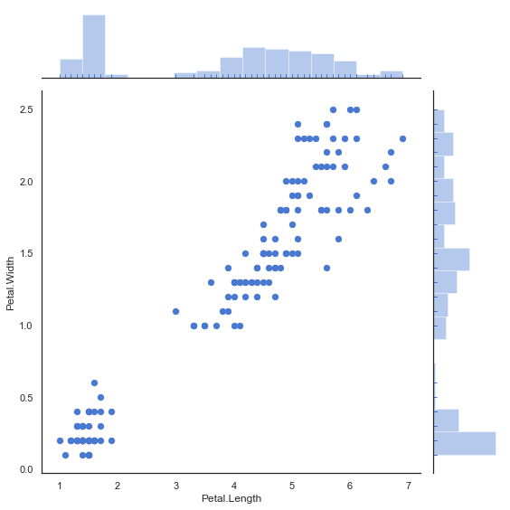
조인트 플롯
# 조인트 플랏

""" scatter plot 2: joint plot """

sns.jointplot(x = 'Petal.Length', y = 'Petal.Width', kind = 'scatter',
              marginal_kws = dict(bins = 15, rug = True),
              annot_kws = dict(stat = "r"), s = 40,
              height = 8, data = iris)
페어플롯
# 페어플랏, 각 자료에 대한 관계를 살펴보기 좋다
# \ 대각선은 밀도 플롯

""" scatter plot matrix: pair plot """

sns.pairplot(iris, hue = 'Species')

sns.pairplot(iris, hue = 'Species', palette = 'husl')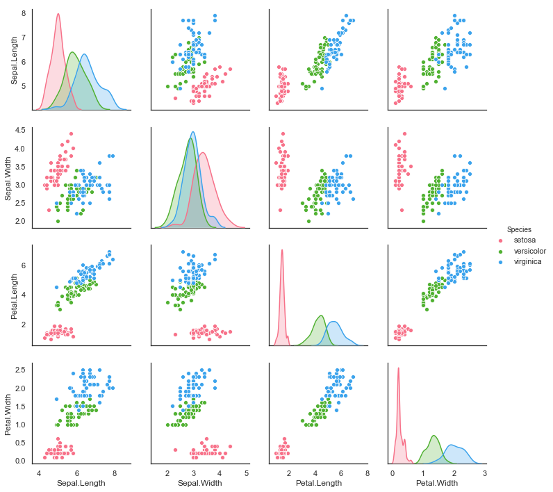
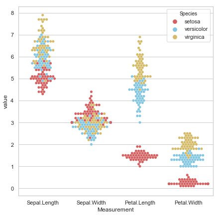
스왐 플롯
"""
스왐 플랏은 새들이 떼지어 다니는 것 같은 형상 때문에 붙은 이름으로
분류(classification) 문제에 효율적이다.
"""


""" scatter plot: swarm plot """
sns.set(style = 'whitegrid', palette = 'muted')

"""
판다스의 melt 메소드는
품종이 맨 앞으로 오고(범주형), 연속형 변수들이 뒤로 가게 한다.
"""

# "Melt" the dataset to "long-form" or "tidy" representation
tidy_iris = pd.melt(iris, 'Species', var_name = 'Measurement')


plt.figure(figsize = (7, 7))
# Draw a categorical scatterplot to show each observation
sns.swarmplot(x = 'Measurement', y = 'value', hue = 'Species',
              palette = ['r', 'c', 'y'], data = tidy_iris)
plt.show()
스트립 플롯
"""
스트립 플롯은 스왐플롯과 유사한 결과를 보여준다.
역시나 분류 문제에 효율적이므로, 적당한 변수를 선택하기에 좋다.
"""


""" scatter plot: strip plot """

# Initialize the figure
f, ax = plt.subplots()

sns.despine(bottom = True, left = True)

# Show each observation with a scatterplot
sns.stripplot(x = 'value', y = 'Measurement', hue = 'Species',
              data = tidy_iris, dodge = True, alpha = .25, zorder = 1)

# Show the conditional means
sns.pointplot(x= 'value', y = 'Measurement', hue = 'Species',
              data = tidy_iris, dodge = .532, join = False, palette = 'dark',
              markers = 'd', scale = .75, ci = None)

# Improve the legend
handles, labels = ax.get_legend_handles_labels()
ax.legend(handles[3:], labels[3:], title = 'Species',
          handletextpad = 0, columnspacing = 1,
          loc = 'lower right', ncol = 3, frameon = True)

plt.show()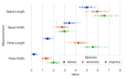
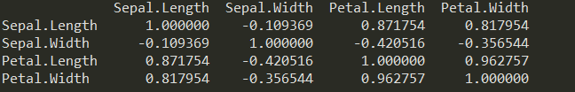
7. 상관계수와 히트맵
상관계수
"""
전통적으로 변수들간의 관계를 식별하기 위해 사용하는 것은
상관계수이다.

그리고 상관계수들 간의 관계를 시각화한 것은
히트맵
"""


# 상관계수
iris.corr()

"""
petal 특성은 서로 양의 상관관계
sepal 은 서로 영향이 적음
sepal.length는 petal 특성들과 양의 상관관계
sepal.width는 petal 특성들과 음의 상관관계
"""
히트맵
""" correlation: heat map """

plt.figure(figsize = (8, 8))
sns.heatmap(data = iris.corr(), annot = True, fmt = '.2f', linewidths = .5, cmap = 'Reds')
plt.show()
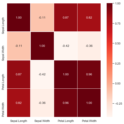
색상이 진할 수록 상관계수가 높은 모습을 보인다.
'Homework > DataMining' 카테고리의 다른 글
| 06. Feature Selection (0) | 2020.05.01 |
|---|---|
| 05. One-Hot Encoding (0) | 2020.05.01 |
| 04. Interpolation / Normalization & Standardization (0) | 2020.04.21 |
| 02. Data Load with sqlite3 (0) | 2020.04.07 |
| 01. Data Exploration & Visualization (0) | 2020.03.24 |
'Homework/DataMining' Related Articles
more


Comments