without haste but without rest
06. Feature Selection 본문
0. 개요
피쳐 셀렉션에 사용할 수 있는 두 가지 방법
1. 분산을 이용하는 방법
- 분산이 작은 데이터는 종속변수에 영향을 덜 줄것이므로 제거한다.
2. 상관계수를 이용하는 방법
- 기준치를 두고 선택한다. ex) 상관계수가 |0.6| 이상
- 예측하고자 하는 변수와 상관계수가 높은 변수일수록 해당 변수에 영향력이 크기 때문이다.
1. 분산을 이용한 방법
###################################################################################
## Feature selection(fitering)
###################################################################################

# load iris dataset
iris = pd.read_csv("./iris.csv")
iris.index.name = 'record'
print(iris.head())

# define columns to filter
cols = ['sepal length in cm',
        'sepal width in cm',
        'petal length in cm',
        'petal width in cm']


# Variance Filtering
"""
분산이 작은 데이터는 종속변수에 영향을 덜 줄것이다. 따라서 필터링한다.
-> variance fileting

"""
###################################################################################

# instantiate Scikit-learn object with no threshold
from sklearn.feature_selection import VarianceThreshold
selector = VarianceThreshold()

# prefit object with df[cols]
selector.fit(iris[cols])

# check feature variances before selection
print(selector.variances_)

# set threshold into selector object
selector.set_params(threshold = 0.6)

# refit and transform, store output in out_sel
out_sel = selector.fit_transform(iris[cols])

# check which features were chosen
print(selector.get_support())	# [True ,False, True, False] = 0, 2


# filter in the selected features
iris_sel = iris.iloc[:, [0, 2]]
print(iris_sel)

# add labels to new dataframe and sanity check
iris_sel = pd.concat([iris_sel, iris[['species']]], axis = 1)
print(iris_sel.head())
2. 로지스틱 회귀 - 분류 문제 (분산 필터링 X vs 분산 필터링 O)
## Logistic Regression
## 필터링을 하기 전 로지스틱 회귀
## 전체 속성을 이용해서 분류를 하는 케이스
###################################################################################

from sklearn.linear_model import LogisticRegression

X = iris.iloc[:, :4].values
print(X)

y = iris.iloc[:, 4]
print(y)

logistic = LogisticRegression(random_state = 0).fit(X, y)
logistic.predict(X)

logistic.predict_proba(X)

logistic.score(X, y)

# score = 0.97


# Logistic Regression:  Variance filtering
# 분산으로 필터링을 하고 로지스틱 회귀
# 분산이 0.6 이상인 속성들로만 예측하는 케이스
###################################################################################

X = iris_sel.iloc[:, 0:2].values
print(X)
y = iris_sel.iloc[:, 2]
print(y)

logistic = LogisticRegression(random_state = 0).fit(X, y)
logistic.predict(X)

logistic.predict_proba(X)

logistic.score(X, y)

# score = 0.96


"""
분산을 필터링한 모델이 스코어가 1프로 낮지만,
더 심플하고 차이가 심하게 나지 않으므로 후자가 더 좋은 모델이라고 할 수 있다.
"""
3. 상관계수를 이용한 피쳐 셀렉션
## Correlation
## 상관계수를 이용하는 피쳐 셀렉션
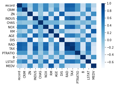
## 상관계수 히트맵 그리기
###################################################################################
# import matplotlib for access to color maps
import matplotlib.pyplot as plt
import seaborn as sns
# load boston dataset
boston = pd.read_csv("./boston.csv")
boston.index.name = 'record'
# find correlation with pandas ".corr()"
cor = boston.corr() # 상관계수
# visualize with Seaborn heat map, color map = Blues
sns.heatmap(cor, annot = False, cmap = plt.cm.Blues)
plt.show()
# get correlation values with target variable
cor_target = abs(cor['MEDV'])
print(cor_target)
# choose features above threshold 0.6
selected_cols = cor_target[cor_target > 0.6]
print("selected columns, correlation with target > 0.6")
print(selected_cols)
selected_cols.index
# filter in the selected features
boston_sel = boston[selected_cols.index]
print(boston_sel.head())
"""
보스턴 데이터 셋에서 MEDV 속성과 상관계수가 |0.6| 이상인
속성들을 걸러내는 작업
"""
4. 회귀분석 - 예측 (상관계수로 필터링 O vs 상관계수로 필터링 X)
## Regression : corr filtering
## 상관계수로 필터링한 데이터들로 회귀분석
###################################################################################

from sklearn.linear_model import LinearRegression

X = boston_sel.iloc[:, 0:2]
y = boston_sel.iloc[:, 2]

reg = LinearRegression().fit(X, y)

reg.score(X, y) # the coefficient of determination

print(reg.coef_)	# 가중치

print(reg.intercept_)	# 절편

## 0.6

## Regression : all
## 필터링 하지 않은 데이터들로 회귀분석
## 하지만 이런 경우 다중공선성의 문제가 발생할 수 있다.
###################################################################################

X = boston.iloc[:, 0:14]
y = boston.iloc[:, 14]

reg = LinearRegression().fit(X, y)

reg.score(X, y) # the coefficient of determination

## 0.74


"""
필터링한 모델의 정확도가 더 낮지만 변수 두개로 60프로 정도의
정확도를 보인다는 것이 강점
"""'Homework > DataMining' 카테고리의 다른 글
| 08. Clustering - K-means, Hierarchical (0) | 2020.05.12 |
|---|---|
| 07. PCA(Pincipal Component Analysis) (0) | 2020.05.05 |
| 05. One-Hot Encoding (0) | 2020.05.01 |
| 04. Interpolation / Normalization & Standardization (0) | 2020.04.21 |
| 03. Visualization with Seabron (0) | 2020.04.14 |
'Homework/DataMining' Related Articles
more


Comments